For some time already, we have the Klippel Nearfied Scanner in our lab. Even so, we got our anechoic- and reverberant room, the scanner is a brillant way to generate a full set of data within a few hours, letting the scanner do its work fully automatically.
Here are some typical results of such a measurement session.
It’s not a secret that dealing with cabinet vibrations is a big thing here at Fink Audio-Consulting. Now that everybody managed to make the speaker drivers better and better, cabinet vibrations are a lot easier to detect. The “nice” masking effect of IM and harmonic distortion is not longer there, so we are able to detect the nasty resonances of real world cabinets.
A few methods have been developed over the last years to control, damp and shift cabinet resonances. Sure, you can go the WILSON way and make your speakers 100kg heavy, but for cheaper speakers this does not work of course.
So what is the best way? How much resonances can we accept? Is it frequency dependent? Yes, it is. Reading the research results of the BBC, you will notice that they found cabinet resonances in the higher midband are evil. But the typical well braced cabinet gives you resonances in the 800Hz-2kHz region. Not very nice as it adds roughness to voices and some unpleasant forward presentation. It’s better to allow the cabinet resonances below 400Hz – this adds some warmth to the performance and can sound a lot more musical.
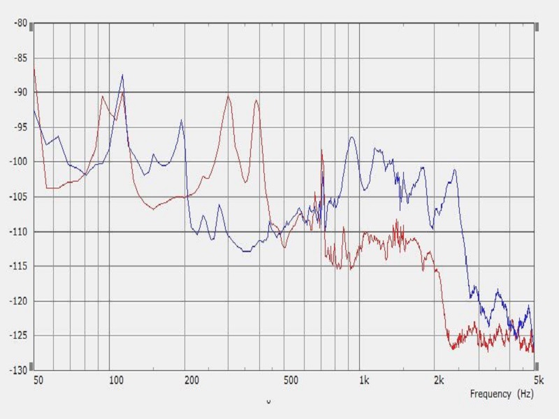
Here ia a comparison between two different cabinet concepts:
The blue line shows cabinet vibrations (one side panel) of a well respected British speaker with a lot of bracing. The bracing is not directly connected to the walls, but has a layer of rubber in between. The cabinet is relatively heavy and feels very solid.
The red speaker shows the side panel of a similar sized speaker – made for another British brand. This speaker is only lightly braced, but uses a sort of sandwich construction with 2 layers of MDF and a lossy layer in between.
As a result we see two complete different philosophies: The blue speaker is very well damped between 200Hz and 500Hz. Above 800Hz, the level goes up stays high up to 2.5kHz.
The red speaker got the maximum output at 300 and 400Hz, drops after 500Hz (the peak on both speakers at 700Hz is the stand) and stays very low up to 2 kHz.
Funny enough, you can hear the same thing listening to the speakers: The blue one is very tight, just a bit lean on lower midband and a shows a forward imaging with flat, but wide sound stage.
The red speaker got definitely more warmth with a very open, natural midband character. The image is completely different. It is not as wide as the blue speaker, but with much deeper soundstage and realistic rendering.
Our development shows that cabinet vibrations not only disturb the midband character, but also shift image around. Just make a simple experiment yourself that I learned from fellow Stephen Harris (Audioplus UK): Listen to a bookshelf speaker on a stand and concentrate on the height of the soundstage. Now take a book or something similar and place it on top of the speaker. In most cases you will immediately notice that the soundstage goes up. What is happening? Well, the book reduces the output of the top panel. The same thing happens with well controlled and damped cabinets: The soundstage is more realistic and not influenced by peaks and dips radiated from the cabinet panels. Not to forget the more relaxed and natural midband 🙂
More to come..
Essen, 24.11.2014 Markus Strunk and Karl-Heinz Fink
In addition to our POLYTEC Laser Scanner, we got the Klippel Laser Scanner recently. Why? Well, the Klippel device uses a Triangulation Laser and can output dimensions. It also couples the measurements to the surrounding air and allows to predict SPL including directivity – with a simple click only.
Here is what you get as animated picture:
Moving cone at 4347Hz
You can also have a look at the profile and here it’s easy to spot the cone/surround junction to be the area to work on:
Cone profile at 4347Hz
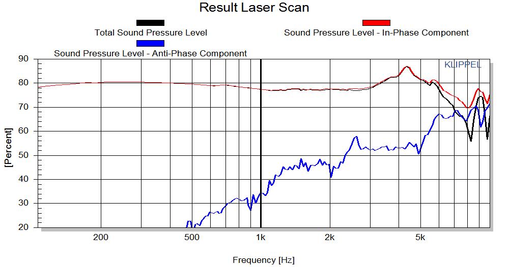
A really nice feature is the option to separate the part of the cone that vibrates in phase and the part that is not in phase and of course the result of both. This option really helps to understand a response curve of a speaker:
Last,but no least it is possible to show radial modes and circular modes in different animations. Below is the circular mode of the driver. As you can see, there is a little bit of a Rocking Mode visible:
Whenever we at FAC design a subwoofer, we test after finishing the equalizing what the loudspeaker does at higher levels. The best method is to do a compression measurement. During this measurement, the input level of the subwoofer is increased and we check if the output level changes follows
A subwoofer after filtering
If you normalize the results to the starting value, you can get a nice picture of what the sub does in real life.
Compression test with the subwoofer shown above
There are two obvious sources of compression. First of all – in case of a ported design- the port starts to fail at higher levels due to too high air velocity, with the result that the region around the tuning frequency does not go loud enough.
The second effect is the thermal compression. The coil get’s hot, therefore the resistance rises and the result is a lower level.
But if you carefully compare the response curve of the compression measurements, you see that there is a difference. Even so the “static” measured curve looks flat, ALL compression curves – even the low level ones – show some slightly falling character.
So what happened? Well, in case of this particular measurement, the driver is measured at each individual frequency with all the defined level steps. During that period from small voltage to larger voltage, the temperature rises in the voice coil. When jumping to the next frequency, even at the lowest level, the coil is still hot and so the level is slightly reduced. So far, so good, but due to the impedance curve of the subwoofer, this change in level is not constant over frequency. At the impedance peak around 60Hz, the level difference is much smaller. As a result, this level stays more or less even at higher levels, but above and below, the levels goes down, depending on the temperature of the voice coil.
Impedance of Subwoofer without amplifgier
One the measurement below the following test was done: The green curve shows the standard measurement with a relatively low input level of 0.1V. The red one was done again with 0.1V just after finishing a high level faster sweep with 1.5V. The blue curve shows the same, but this time the high level sweep was done slower to give the coil time to heat up.
One could say this is a fault in the measurement and maybe it needs to be changed to avoid that effect, but if demonstrates nicely what happens in the real world with music or a movie. The coil get’s hot during peaks or heavy bottom end and the resulting response curve is changing. For the design process it means to make sure that from the frequency of the high impedance peak, the “static” response rises slightly around 1dB. That means in real live you get a better balanced behavior.
Compression curves after filter modification
This modification might not make a good subwoofer starting with a bad one, but a carefully look at thermal compression cannot be wrong and it is not a lot more work to take care about the effects.
Thanks to Christian Gather, who made all the measurements and had the initial idea.
Nearly everybody in our industry knows the AES article about nearfield measurements of Don B. Keele introduced in 1974. In his article, he described a way to make a nearfield measurement of a speaker and he compared it with the farfield response of the same speaker. He came to the following conclusion:
Based on that conclusion, a lot of speaker engineers started using the nearfield measurement of a woofer to stitch it together to a farfield measurement made in a anechoic chamber. This was to overcome the limitations of a real world chamber at low frequencies (below 100-200Hz, depending on room size).
Unfortunately, many did not take into account that a nearfield measurement of a todays size loudspeaker does not represent the farfield result even at low frequencies. The limited front baffle has a major effect on the farfield response.
Funny enough, Mr. Keele included that already in his article:
He mentioned “half space” and that means the speaker should be on a big baffle. But normally a speaker box is measured free standing in 1m distance, and that’s full space. The difference to a half space measurement is huge!
Mr. Keele showed clearly what he measured – you just have to carefully look at it.
The speaker tested in this example was a 4.5″ in a cubic enclosure of roughly 22cm. The farfield result can be seen in measurement a. The nearfield result in in b. In c, the small enclosure was mounted into a bigger baffle of roughly 1.2×2.4m to “support” the the small enclosure. Only now, nearfield and farfield looked similar.
It can be said that the work of Mr. Keele is still valid and true, as long as everybody understands that nearfield and farfield measurements are only comparable if you have made the farfield under half field field conditions or found a method to recalculate a nearfield measurement into a farfield version.
A good exercise to understand the influence of the baffle to the farfield response curve is the nice little program called “The Edge”. This free goodie can be used to calculate a baffle step compensation, but also shows nicely the effect a limited baffle size has already at low frequencies. There are other nice free programs at the same site – it’s worth going there.
All quotes of Mr. Keele have been taken from his original article, the two pictures of EDGE can be found on the web site of Mr. Tolvan. Part 2 will show a way to re-calculate nearfield measurements into farfield versions.
Let us test your drive units. We tell you how good they are and we know how to make them better. Promised.
Analyzing is a big part of our business. We therefore have a lot of special equipment available for testing purpose.
Klippel Analyzer for Transfer function measurement in anechoic chamber
Klippel Analyzer for testing dynamic behaviour and static parameters
Polytec Scanning Vibrometer to monitor cone and surround movement
Once we have analyzed the driver, we can help to optimize it by:
Designing a new magnet system, using latest simulation methods made by powerful commercial and homemade software
Developing new soft parts like Cones, Surrounds and Spiders with modern FE/BE simulation. Material property can be measured at our place.
Performing listening tests, done by very experienced engineers and music lovers.
Interested? Give it a try. The first driver test is on us 🙂
We use cookies to ensure that we give you the best experience on our website. If you continue to use this site we will assume that you are happy with it.Ok